Explore, Exploit, and Explain: Personalizing Explainable Recommendations with Bandits

Summary

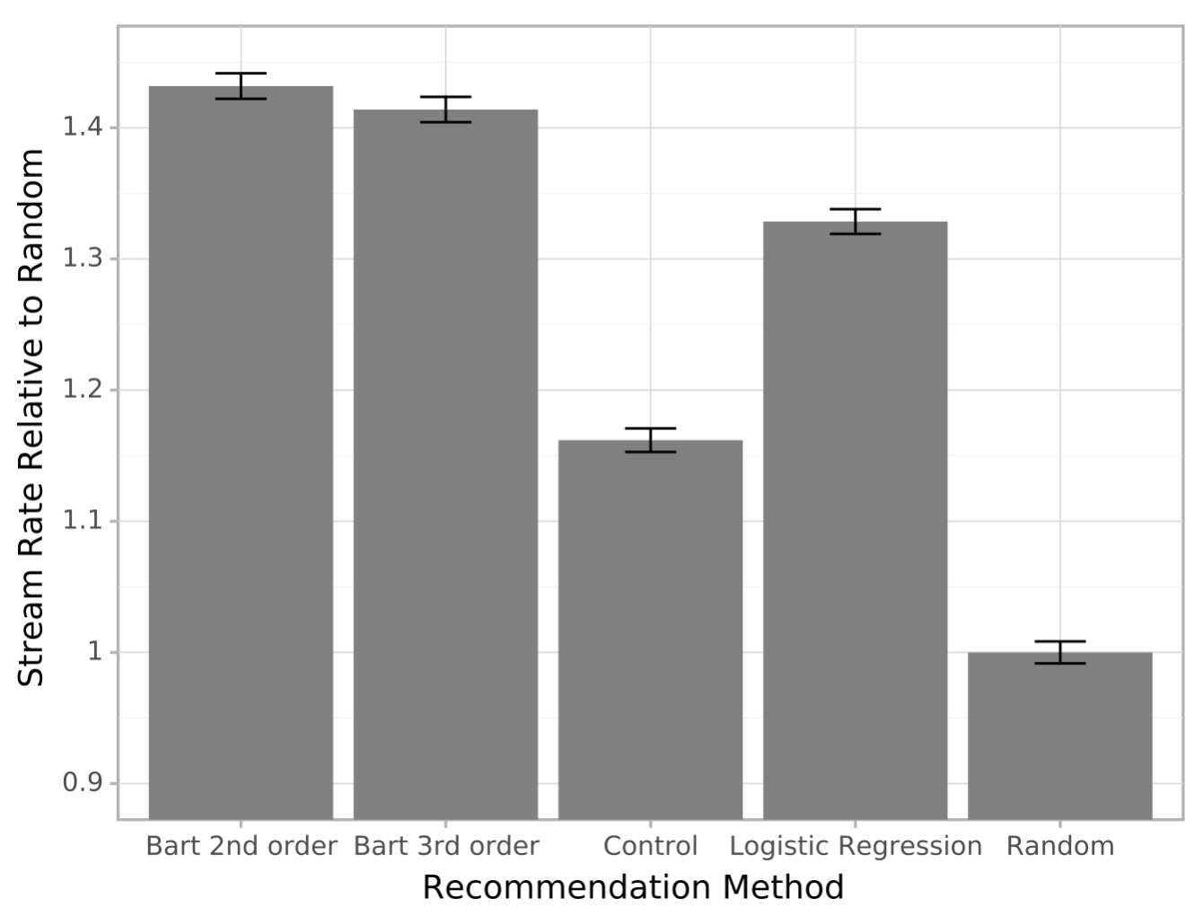
In our recent RecSys publication, we propose a bandit method for personalizing explainable recommendations (e.g. cards on a grid with shelf titles). Our method provides a way of approximating online metrics using counterfactual evaluation with grid-based propensities. Experiments on the Home page of Spotify show a significant improvement in stream rate over non-bandit methods and a pretty good agreement in offline and online ranking of approaches.

Here are some associated resources:

J. McInerney, B. Lacker, S. Hansen, K. Higley, H. Bouchard, A. Gruson, R. Mehrotra. Explore, Exploit, Explain: Personalizing Explainable Recommendations with Bandits. In ACM Conference on Recommender Systems (RecSys), October 2018.

Slides | Poster | Blog | Paper

motivation

I start by describing the motivation for bandits in recommendation then describe how explained recommendations are now a common use case in modern recommender systems.

Why the Rich Get Richer In Content

A small number of content producers dominate consumption in culture. This happens wherever exposure (e.g., word of mouth, media coverage, recommendation algorithms) is higher for popular producers than less popular producers. More popularity leads to greater exposure and greater exposure leads to more popularity (see Fig. 1). This is known as the Matthew effect (biblical reference) or the Pareto principle [Juran, 1937]. The way this plays out in recommendation algorithms is interesting and worth diving into next.

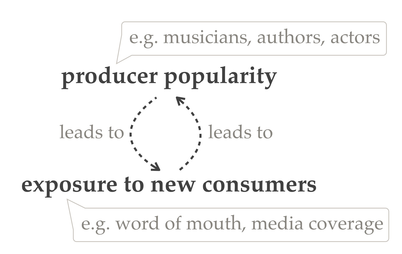
Figure 1. More popular content producers receive greater exposure which feeds their popularity.

A Causal Diagnosis for Filter Bubbles in Recommendation

Filter bubbles occur when you train a model on user response data gathered by a recommender [Chaney et al., 2018]. The problem originates because items receive different levels of exposure, which biases the learnt relationship between treatment (i.e. recommended item) and response (i.e. observed relevance) [Liang et al, 2016]. Fig. 2 gives a schematic of the way that most recommenders in production across industry are deployed. An alternative way to describe the problem is with Pearl’s do-calculus: in training a model of user response given recommendations, our model is biased by the back-door path that goes via the contextual information (e.g. the user history or user covariates).

Figure 2. Feedback loops in existing recommender systems result in biased models.

This motivates the need for contextual bandit approaches that explore the item space sufficiently and correct for the bias in the training objective.

Contextual Bandits for Recommendation

To understand the role of bandits in all this, it helps to introduce the notion of recommender uncertainty (see Fig. 3). When all a recommender can do is either exploit (i.e. recommend) or ignore (i.e. not recommend) an item, the recommendation system ends up ignoring potentially relevant items. This happens to due to the fact that it only ever has access to finite data about user responses.

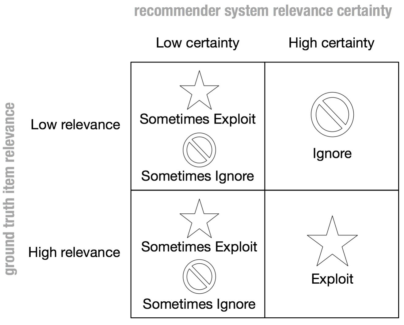
Figure 3. When a recommender is uncertain about an item relevance to a user, all it can do is either explore or ignore.

Wouldn’t it be nice if our recommender could also recommend items on an exploratory basis when it is uncertain about its relevance? This motivates using a contextual bandit (see Fig. 4) [Sutton & Barto, 1998]. The type of bandit we focus on here is a stochastic policy contextual bandit because it affords importance sample reweighting (described in the “Counterfactual Training” section).

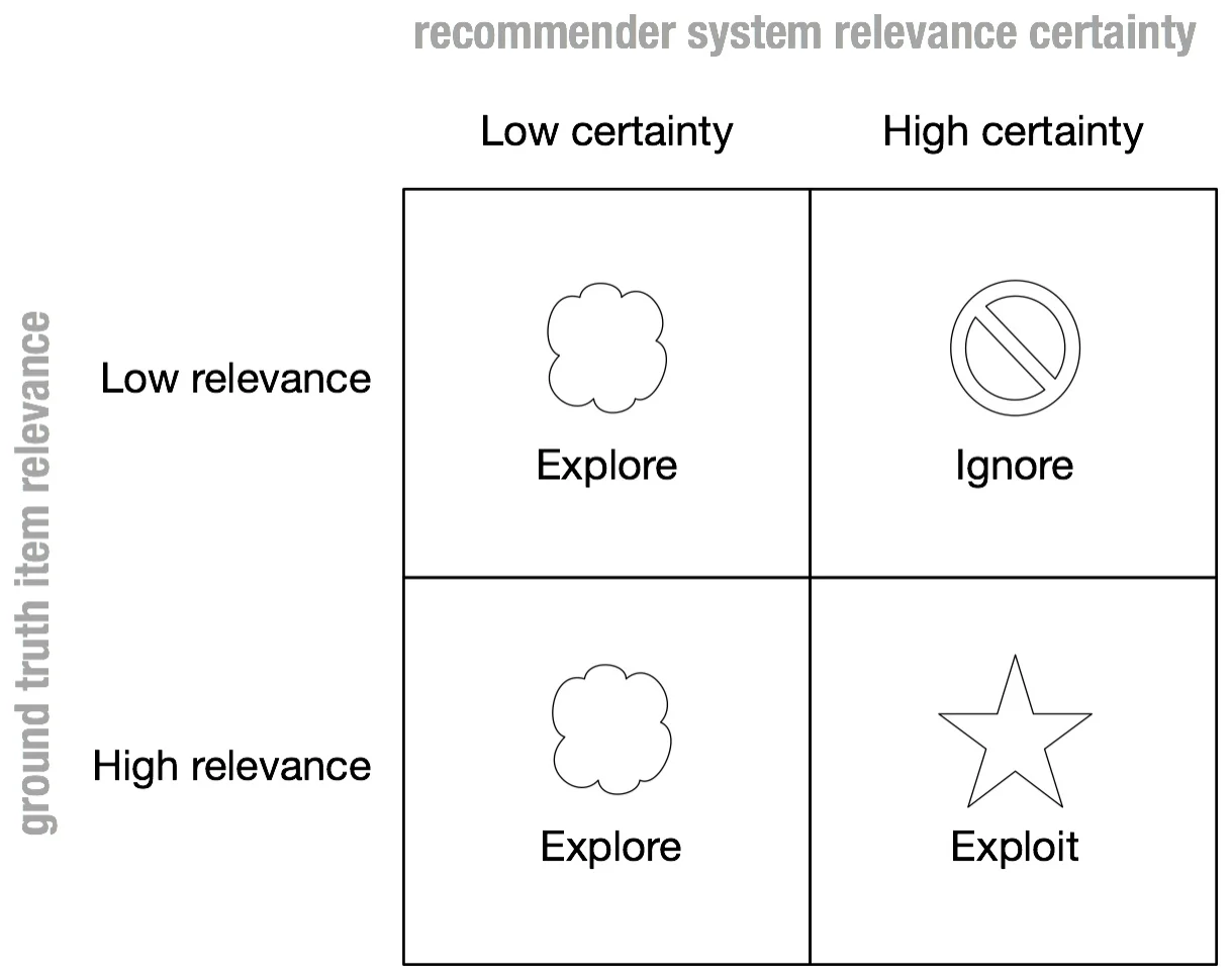
Figure 4. When a bandit recommender is uncertain about an item relevance to a user, it can make sure to explore those items.

Recsplanations

The final piece of the motivation relates to explained recommendations, or recsplanations (a term coined by Spotify’s Paul Lamere a few years ago). Recsplanations are now a common way for a recommender to tell a user why they are being recommended a particular item. They are often manifested in a shelf interface: e.g. on the Spotify home page on the mobile app you see playlists arranged on shelves, and each shelf has a title or theme that tells you a bit about where the recommendations come from (“based on your recent listening”, “because your friends like”).

Figure 5: example of a shelf interface recommender.

The research question is: how can we extend the bandit approach to recsplanations?

Bandits for Recsplanations as Treatments (Bart)

Bart consists of a reward model, a stochastic policy, a counterfactual training method, and a propensity score scheme. I discuss each choice next.

reward model

The job of the reward model is predict the user response given a context and recommended item:

$$\mathrm{predicted \; reward\;} = \mathbb{E}_{p_\theta(R | A, X)}[R]$$

where X is the context (e.g. recent user listening, region, platform), A is the recommended item, R is the user response (e.g. stream = 1, no stream = 0), and \( \theta \) are a set of model parameters.

What makes a good reward model? That depends on the kind of data and problem. For recommendation, it helps to use methods that do not fold under data sparsity, since there may only be a few responses per user for you to train on. For our experiments, we focused on the class of factorization machines [Rendle, 2010].

stochastic policy

How you explore items with an uncertain reward is also a design choice. Given that exploration is wasteful it makes sense to focus it where there is the most uncertainty. Ideally, as our recommender gains confidence in the quality of some items it explores them less. For simplicity we chose epsilon-greedy, which takes the following form:

$$\pi(A | X) = (1-\epsilon) + \frac{\epsilon}{|\mathcal{A}|} \mathrm{\;when\;}A=A^*$$

$$\pi(A | X) = \frac{\epsilon}{|\mathcal{A}|} \mathrm{\;otherwise} $$

Could we have used upper confidence bounds (UCB) or Thompson sampling? UCB is a deterministic policy so is not compatible with the importance reweighting trick we are about to use. Thompson sampling requires an accurate quantification of uncertainty in the reward prediction, so we leave that for future work.

Counterfactual Training

Our ideal training objective is on data collected through a randomized controlled trial:

$$\mathbb{E}_{X, A \sim \mathrm{Uniform}(\mathcal{A}),R}[\log p_\theta(R | A, X)]$$

But you can’t always get what you want: users would get dissatisfied if we just recommended them things regardless of relevance. Therefore, our approach is to collected data with a biased policy, \( \pi \) described above, then manipulate the objective such that it approximates the randomized controlled trial:

$$\mathcal{L}(\theta) = \frac{1}{N} \sum_{n=1}^N \frac{\log p_\theta(R | A, X)}{|\mathcal{A}| \pi(a | x)}$$

In fact, we do the counterfactual training using normalized capped importance sampling (NCIS) in order to reduce the variance of the estimator [Gilotte et al., 2018].

Propensity Scores

The novel aspect of the training procedure is how to specify the propensity scores (i.e. the logging policy) and, concomitantly, the stochastic policy on the explanation grid.

Let’s start from what would make our lives easy: given a database of impressions and stream outcomes, the most natural plug-n-play approach is to train on the rows of this database as weighted i.i.d. observations in a classifier (or regressor for continuous rewards). What are the weights? None other than the inverse propensities.

How does that translate into bandit world? It turns out, it is equivalent to filling in slots in two directions with a bandit action in each slot. First, fill up each shelf with a diminishing action space of items, preselected to be relevant to the shelf title (a form of safe exploration):

Figure 6

Figure 7

Second, fill up each shelf with a diminishing action space of shelves.

Why are we allowed to decide the ordering before a single impression has been collected? The reason is because our reward model is only trained episodically: \( \theta \) remains the same therefore we can greedily choose item placements, on the strong assumption that the rewards for each action are independent.

Experiments on the Home Page

We studied a range of settings and compared to a baseline that does not use dynamic ordering of items (control) and a random placement of items. We found a significant improvement when using contextual bandits. Further details around the experimental setup are in the paper.

Conclusions and Future Work

We introduced Bart, a contextual bandit approach to performing exploration-exploitation with recsplanations. There are clearly several extensions to improve the approach. First, the user preference model is amenable to several improvements: it assumes independence of rewards (ruling out rankings that encourage diversity of content), estimates absolute reward when comparative reward (a la LambdaMart) could be more accurate, and it is vulnerable to our definition of user stream as the success metric (why not stream length?). The second avenue of improvement is along whole page optimization lines: can we use the slate method to improve this [Swaminathan et al, 2018]?

References

[Chaney et al., 2018] Chaney, A. J., Stewart, B. M., & Engelhardt, B. E. (2018, September). How algorithmic confounding in recommendation systems increases homogeneity and decreases utility. In Proceedings of the 12th ACM Conference on Recommender Systems (pp. 224-232). ACM.

[Gilotte et al., 2018] Gilotte, A., Calauzènes, C., Nedelec, T., Abraham, A., & Dollé, S. (2018, February). Offline A/B testing for Recommender Systems. In Proceedings of the Eleventh ACM International Conference on Web Search and Data Mining (pp. 198-206). ACM.

[Juran, 1937] Juran, J. (1937). Pareto principle. Juran Institute.

[Liang et al., 2016] Liang, D., Charlin, L., McInerney, J., & Blei, D. M. (2016, April). Modeling user exposure in recommendation. In Proceedings of the 25th International Conference on World Wide Web (pp. 951-961). International World Wide Web Conferences Steering Committee.

[Pearl, 2009] Pearl, Judea. Causality. Cambridge University Press, 2009.

[Rendle, 2010] Rendle, S. (2010, December). Factorization machines. In Data Mining (ICDM), 2010 IEEE 10th International Conference on(pp. 995-1000). IEEE.

[Sutton & Barto, 1998] Sutton, Richard S., Andrew G. Barto, and Francis Bach. Reinforcement learning: An introduction. MIT press, 1998.

[Swaminathan et al., 2018] Swaminathan, A., Krishnamurthy, A., Agarwal, A., Dudik, M., Langford, J., Jose, D., & Zitouni, I. (2017). Off-policy evaluation for slate recommendation. In Advances in Neural Information Processing Systems (pp. 3632-3642).